Visualizing time series inputs for RNNs

Motivation

My background in deep learning stems from building computer vision systems, so I wanted to expand my horizons and develop a more holistic view of the field. This search led me to the excellent Learning Deep Learning book by Magnus Ekman and published by NVIDIA. With the rise of Transform-based networks, it became clear that it was time to become comfortable with sequential data.

The book Learning Deep Learning introduces recurrent neural networks with an example of a network that learns to predict US book sales prices using historical sales data. The data consists of the combined monthly sales of US booksellers dating back to 1992 up to 2020.

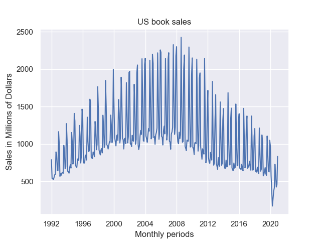
The data contains 348 months of sales. If you squint, you can see repeating patterns showing the seasonality of the sales. The next question is, how can we present this to a recurrent neural network?

Preparing the data

Pictorially, we can visualize the data as follows.

In our case, n is 348. Next, we want to create training, validation, and testing splits. Note that in the book, Ekman uses an array called test for validation. I will refer to this as the validation set, for which it is used, but the example code on his GitHub uses the test naming. An 80% split yields a training set of 278 examples and a test set of 70 examples.

At this point, the book discusses different options for preparing the training set. If we wanted to predict m1, we would have empty input. When predicting m2, we would have m1 as historical data. With mi, we have m_i-1 prior points. While we could feed this to a network, training would be inefficient. Frameworks like PyTorch and TensorFlow require batches with a consistent length.

The above diagram shows how we can require a minimum amount of history without losing potential training examples. In the code, we need 12 months of history. This leaves 278 – 12 = 262 months to build our training examples.

Building training data

Ekman provides the following code for building the training data set:

# Create training examples.
train_months = len(train_sales)
train_X = np.zeros((train_months-MIN, train_months-1, 1))
train_y = np.zeros((train_months-MIN, 1))
for i in range(0, train_months-MIN):
    train_X[i, -(i+MIN):, 0] = train_sales_std[0:i+MIN]
    train_y[i, 0] = train_sales_std[i+MIN]

He recommends tracing through the code to understand this loop better. I wanted to provide a picture to help illustrate what the loop does.

The code starts by allocating and zero-initializing a tensor with the shape 262 x 277 x 1. The zero initialization corresponds to the padding value. We have up to 277 data points for each training example. Why 277? We take the most recent point and make it the y value. The one corresponds to our monthly sales dimension, but we could also include other data for a monthly measure of consumer optimism.

When we enter the loop, we see it building the structure in the above illustration. The right-most edge of the array represents the most current monthly data, while the left-most edge represents the oldest time points. The shaded area shows the minimum required history. The previous monthly target becomes the most recent data point with each loop iteration.